Not taking Add Math and not having the slightest bit of differentiation in IGCSE unlike the syllabus now, I was terrified of studying calculus as I came in like a clean slate without any prior knowledge. Of course, I’ve always heard about how arduous it was from my seniors and classmates and noticed how the atmosphere went cold at the word “calculus”, but calculus in my opinion at least, isn’t as difficult as what I had expected dare I say compared to cough complex numbers. I enjoy doing calculus now to some extent because the problem is stated just as it is, leaving little room for misinterpretation.
Riemann Sum
Source: https://www.youtube.com/watch?v=FRpikUS2v-g&feature=youtu.be
The video above delves into and explains the Riemann Sum pretty well hehe. Butttt I will give a summary of the main concept anyways.
So if you were lazy to watch that almost 30 minute video, you might still be wondering what Riemann Sum is.

If you were told to find the area of ACDB, what would you use? No regular shape would fit that shape to give us an exact formula to find this area. Instead we can approximate the area obtained by summing up the areas of rectangles that try to approximate the shape of this curve in that specific region, which is what Riemann Sum is all about.
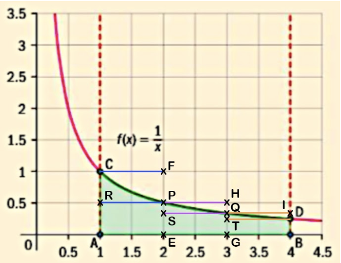
Like in this figure for example, we can split this region into three rectangles above the curve and below the curve. Rectangles above the curve include rectangles ACFE, EPHG and GQIB which when added together gives the value of the upper sum. This is because it gives an area bigger than the actual area of ACDB as seen by part of the rectangle above the curve. Upper sum is also known as left Riemann sum, named so because the upper left corner of the rectangles used touches the curve.
Similarly, rectangles below the curve include rectangles AEPR, EGQS and GBDT which when added together gives the value of the lower sum. This is because it gives an area smaller than the actual area of ACDB as seen by part of the curve not covered by the rectangle. Lower sum is also known as right Riemann sum, named so because the upper right corner of the rectangles used touches the curve.
The actual area of ACDB is going to be in between this upper sum and lower sum and can be approximated further to be equal to the average of these two sums.
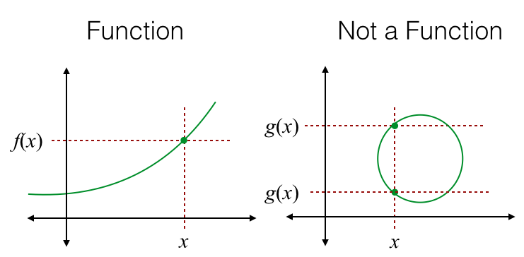
Note that the area you want to find has to be defined in the sense that it is bounded between for example two vertical lines, f(x) and the x-axis as in this case.

Finding the upper and lower sum was repeated again but with 6 rectangles each above and under the curve instead of 3. When this is done a slightly different value is obtained as seen in the video. Butttt, if you compare the average of the upper and lower sum using 6 rectangles to the one with 3 it will be closer to the actual value under the curve found with definite integral.
Now, what if we have 12 rectangles or 24 or even 100? We can generalize the method done to find the area with 3 and 6 rectangles in the following formula. Take note this specific formula is only applicable for decreasing functions and would need to be switched in the case of an increasing function.

To make things more clear, X sub 0 would be point A in Figure 3 and point B would be X sub 1 and so on.
Since Riemann sum is just an approximation, if we wanted to find the exact area under a curve we need to utilize the concept of limits. To do this, the width of each rectangle must approach zero, which in turn means that the number of rectangles n that make up the region would approach infinity. All of the above has now helped us derive, or better said define the Riemann Sum to find the area under the curve, which is:

This equation can be rewritten as what is globally known as the definite integral that gives us the area between the x-axis and the curve over a defined interval [a, b]:

You might have noticed that using a definite integral is essentially the same as following Riemann’s sum using an infinite amount of shapes (rectangles) and an infinitely small value for the width of each rectangle.
The Fundamental Theorem of Calculus
Differential and integral calculus are related to each other, although they might seem unrelated at first. This relationship is very important as seen from the self-explanatory title of this theorem. We will see how they are related in the following parts.
First Theorem
If f is continuous on [a,b], then the function defined by
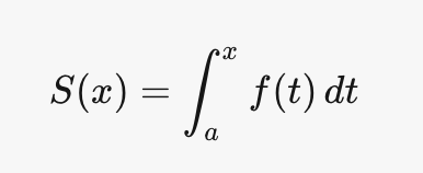
Source: (“Fundamental Theorem of Calculus | Brilliant Math & Science Wiki”, n.d.)
is continuous on [a,b] and differentiable on (a,b), and S′(x)=f(x).
In simpler words, integration is the opposite of differentiation. This can be more clearly rewritten as below:

Source: (“Fundamental Theorem of Calculus | Brilliant Math & Science Wiki”, n.d.)
Second Theorem
If f is a continuous function on [a,b], then

Source: (“Fundamental Theorem of Calculus | Brilliant Math & Science Wiki”, n.d.)
where F is an anti-derivative of f, i.e. F′=f.
Thus, from these theorems we see that differentiation and integration are indeed interrelated with each other.
International Mindedness
Before formulas were invented to calculate the area under a function, this concept was explored by the ancient Greek astronomer Eudoxus using the method of exhaustion. He attempted to find the volumes and areas by splitting up the region into an infinite number of divisions. This method was further applied by Archimedes in the 3rd century BC to find the area of shapes like circles, ellipses etc.
Much later on, the relationship between calculus and integration was made by Liebniz and Newton independently during the late 1600s and early 1700s. Both of them have made equally important contributions to the mathematics field (Rosenthal, n.d.).
Real Life Applications
Calculus is used everywhere especially by engineers. There is a strong connection between physics and calculus.
- Before cars can be sold, the center of mass needs to be checked using integration. This aspect is important to check as it determines the safety of a car on different types of roads and speeds (“Center of mass and gravity”, n.d.).
2. To model predator-prey populations can be done with the Lotka-Volterra equations which are differential equations (“Lotka-Volterra Equations — from Wolfram MathWorld”, n.d.).
3. To determine the rate of a chemical reaction using integration (Reyes, n.d.).
4. To study the spread of an infectious disease which relies immensely on calculus. It can even determine how far and fast a disease is spreading amongst other uses (“Using Calculus to Model Epidemics”, n.d.). This is very important especially in today’s world where Covid-19 is still rampant.
IB Learner Profiles
Communicators – Throughout this whole investigation all the way to the finishing touches leading up to our presentation, communication was an important aspect in completing our work. This learner profile allowed us to delegate tasks and correct each other’s mistakes.
Balanced – We made sure to split up the work in a fair way. More than that, doing the toolkit we made sure to not do all the work the night before and did it in small increments which ensured that we were able to get a good nights rest and have some personal time.
Risk-taker – Even though one of our teammates wasn’t able to present abruptly, we thought of a way to overcome this. Although it was a challenge to present with 3 people rather than 4, we found a way to overcome this issue when we decided that prerecord the voice.
Thinkers – One part of the toolkit which required of me to come up with a generalized formula made me think deeply. It took me a while to get the solution but once I did it it felt like an aha moment.
Open-minded – There were probably times in this toolkit where each one of us made mistakes, at least I know that I made some. Instead of looking down on these mistakes, I took people’s thoughts on what I did wrong and made it into a learning experience to grow from.
Sources
Center of mass and gravity. Retrieved 1 November 2020, from http://ruina.tam.cornell.edu/Book/COMRuinaPratap.pdf
Fundamental Theorem of Calculus | Brilliant Math & Science Wiki. Retrieved 1 November 2020, from https://brilliant.org/wiki/fundamental-theorem-of-calculus/
Lotka-Volterra Equations — from Wolfram MathWorld. Retrieved 1 November 2020, from https://mathworld.wolfram.com/Lotka-VolterraEquations.html
Reyes. Differential and Integrated Rate Laws. Retrieved 1 November 2020, from https://laney.edu/abraham-reyes/wp-content/uploads/sites/229/2015/08/Differential-and-Integrated-Rate-Laws1.pdf
Rosenthal, A. The History of Calculus. Retrieved 1 November 2020, from http://people.math.harvard.edu/~knill/teaching/summer2014/exhibits/lagrange/history_calculus_rosenthal.pdf
Using Calculus to Model Epidemics. Retrieved 1 November 2020, from https://homepage.divms.uiowa.edu/~stroyan/CTLC3rdEd/3rdCTLCText/Chapters/Ch2.pdf


